How to use Excel UnPivot Columns for Fact Tables
Being able to transform data in a table from one format to another is one of the most important tasks you have as a data analyst. Excel’s built-in Unpivot functionality can be used to transform data entry tables into fact tables for better data analysis. This comprehensive guide provides step-by-step instructions, making the process of converting Excel tables using Unpivot Columns functionality easy and efficient.
If you have an Excel table built for data entry, it may not be in the best format for data analysis or your data model. Using Query Editor and the function UnPivot Columns, you can keep the original table and create a version that you can use for analysis as a dimensional fact table.
Note: A Sample workbook is available on Github, WorkLifeBalance_Share_UnPivot.xlsx
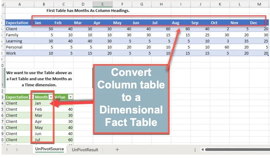
Before and After example.
The table pictured above is set up for easy data entry; however, it could be better for analysis. I want to treat the Expectations and Months as dimensions in queries. This creates more of a StarSchema-type fact table built for analysis in tools like Power BI.
Above are the before-and-after pictures. Before, each column is a month, making data entry easier. Below is a 3-column table that could be used in the analysis. Setting up the dates as columns allows for attaching a StarSchema Data Dimension table.
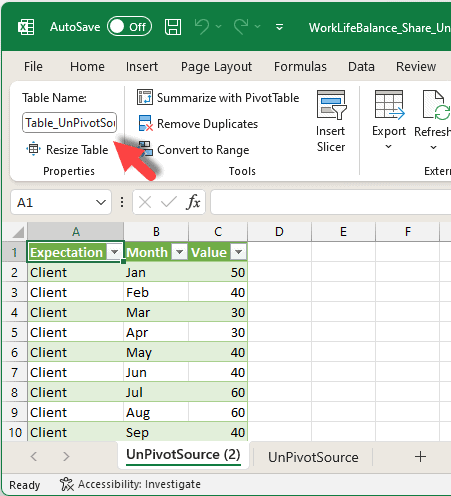
Note that the source range is set up as a table. You can use a range or a table, but setting up your "Tables" as "Tables" in Excel opens up many functionality. See the Post, 5 Steps to Improve Your Excel Data Tables, which includes how to set up a range as a table.
Step 1 - Select Table To Transform With Power Query
It becomes easy to use an easily forgotten set of functionality in Excel. Select the top left column, the Expectations column in this example.
Select the table by selecting the top left Column
As shown below, under the toolbar Data Menu option, there is a section called Get & Transform Data. In that set of options, select From Table/Range. You will notice the popup message that you can use a named range, but it will be converted into a Table.
This brings up Power Query. There are many options for processing your data for loading, but here, we are just going to transform this range.
Step 2 - Select Range and UnPivot
As Pictured below, your selection is brought into the Power Query plugin. In 3 steps;
Select the Columns you want to transpose into 1 Column. Select the first column, scroll to the end, hold down shift, and select the last column. This will highlight your selection. If you have another sample, you would do this for each column you want to create.
On the top menu, select Transform.
Select UnPivot Columns
Step 3 - Results
As shown below, you now have Power Query showing the results. Is what you were looking for,
Double-click on the Month column heading and change the name from "Attribute" to Month.
Click on Close & Load to bring up a dialog.
This adds a worksheet with the results to be used as a data source, leaving your original untouched.
Close & Load
Step 4 - New Table is Updateable With Refresh data
The main benefit of doing this is that it allows you to change values in the original table, and the changes flow through to your new table. The following steps are pictured below.
Change a value in the original table, Family Jan, to 500
Go to the New "UnPivot" Table
Select "Refresh" on the toolbar, and you will see that the value on the Family, Jan Cell, is now 500.
Conclusion
This quick tutorial shows how to take an Excel sheet used for data entry and convert it to a Fact Table by using the UnPivot Columns functionality in the Data Query tools in Excel.
Let me know what you think. Does this fit into your workflow? Let me know if you have any tricks you use.
FAQ
Q1 - What is the purpose of using the Unpivot Columns functionality in Excel?
The Unpivot Columns functionality in Excel transforms data set up for data entry into a format more suitable for data analysis. This is particularly useful when you want to convert your Excel tables into dimensional fact tables for analysis in tools like Power BI.
Q2 - How can I select the range to Unpivot in Excel?
To select the range to Unpivot, you need to first select the top left column of your table. Then, under the Data Menu, there is a section called 'Get & Transform Data'. In that set of options, select 'From Table/Range'. This will bring up Power Query, where you can process your data for loading.
Q3 - How do I use the Unpivot Columns function in Power Query?
Once your selection is brought into the Power Query plugin, follow these steps:
Select the columns you want to transpose into one column. Select the first column, scroll to the end, hold down shift, and select the last column. This will highlight your selection.
On the top menu, select 'Transform'.
Select 'Unpivot Columns'.
Q4 - How can I update the new table created using the Unpivot function?
The main benefit of using the Unpivot function is that it allows you to change values in the original table, and the changes flow through to your new table. To update the new table, simply change a value in the original table, go to the new 'Unpivot' table, and select 'Refresh' on the toolbar. The value in the new table will be updated accordingly.
Q5 - Can I use a named range instead of a table for the Unpivot function?
Yes, you can use a named range for the Unpivot function. However, it will be converted into a table in Power Query.
Steve


